

A simple trichromatic camera model
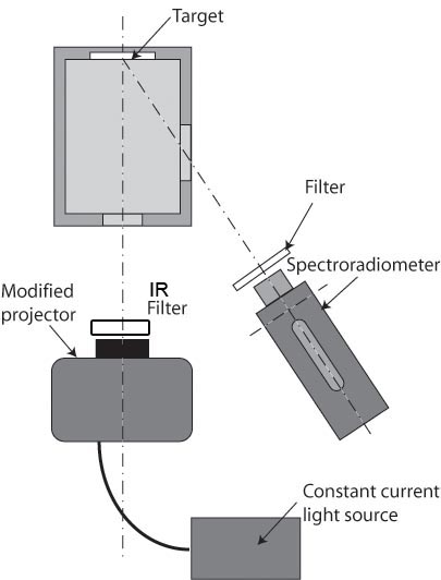 The figure on the left shows a schematic view of the positioning of our spectroradiometer, the light source and the target device. The light source was a modified slide projector fitted with a tungsten-halogen lamp (Osram HLX 64657FGX-24V, 250W). The projector was supplied with constant current (10.00 Amp) provided by a customised power supply (accurate to 30 parts per million in current). In front of the light source there was an Infra-red blocking filter (B+W UV/IR blocking filter 486), to remove all possible traces of IR light from the source. The target was inside a black box with two holes (as seen from the top in the figure). One of the holes was used to let the light from the light source enter the box and the other was used to collect the light reflected from the target at back of the box. The target itself consisted of a thick layer of Cyanoacrylate adhesive powder (Kodak-Eastman "standard white" of 99% reflectance across the visible spectrum) which has a diffuse (Lambertian) pattern of reflection.
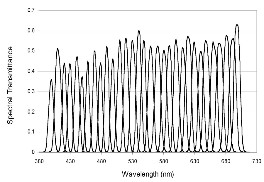
The spectral radiance of the light source and the transmittance of the 31 narrowband interference filters was measured in 1nm steps using this same setup. They span the whole visible spectrum with peaks spaced approximately 10nm and half-bandwidths of less than 5 nm each.
To calculate the energy flux present at the sensor's level, we measured the radiant power (in W.m-2.nm-1.sr-1) and converted it to Joules m-2 using the formula:
| :Equation 5 |
|---|
where R(l) is the spectral transmittance of the filter, I(l) is the spectral radiant power as measured by the spectroradiometer, l represents wavelength, w is the solid angle determined by the camera's aperture and focal length and T is the integration time. All camera-dependent constants were estimated either from the camera's manufacturer's specifications or obtained from the picture's header.
The energy flux actually captured by each sensor is just the above as sampled by the specific sensor's sensitivity. In our calculations we used equations in the discrete form, that is:
 |
:Equation 6 |
|---|
where R, G and B represent the total energy flux captured by each sensor during exposure time T. In the previous equation, all variables are known except Sr,g,b(l), the sensors' spectral sensitivities.
From our previous measures we established that the camera output in grey-levels has a given dependency of light intensity, which expressed for all three sensors has the form:
 |
:Equation 7 |
|---|
where r, g and b are grey-levels of each sensor, R, G and B the energy flux, and a, b and c are the corresponding constants for each sensor.
Combining Equations 6 and 7 we get:
 |
:Equation 8 |
|---|
which is a description of the grey-level values obtained as a funtion of all other varaibles and paramenters. In Equations 8, all parameters a, b, c, and d are unknown but can be approximated from those in Equation 4. We also don't know the shapes of the sensor's sensitivities S(l).
To obtain the unknown parameters of equations 8 we compared the r, g, b values from Equation 8 to those obtained from the original set of 31 photographs (taken though each of the monochromatic filters) and the Macbeth Color-Checker pictures (one rgb triplet for each Color-Checker square). We will refer to these values as ![]() and
and ![]() . By minimizing the differences between these (see equation below) we converge to a set of optimal parematers that explain our results.
. By minimizing the differences between these (see equation below) we converge to a set of optimal parematers that explain our results.
 |
:Equation 9 |
|---|
As a first approximation, we modeled the sensor's sensitivities S(l) as a set of Gaussians whose free parameters were height, peak position and width. The initial a. b, c and d values were those obtained for the luminance case. The values ![]() r,g,b in Equation 9 were minimised, comparing those obtained while photographing the Macbeth card and the chromatically filtered white target (
r,g,b in Equation 9 were minimised, comparing those obtained while photographing the Macbeth card and the chromatically filtered white target (![]() and
and ![]() ) with those obtained theoretically through equation 8 ( r, g, b). From the fitting algorithm we found both the parameters of the equation 7 and the sensitivities S(l) of equation 6.
) with those obtained theoretically through equation 8 ( r, g, b). From the fitting algorithm we found both the parameters of the equation 7 and the sensitivities S(l) of equation 6.
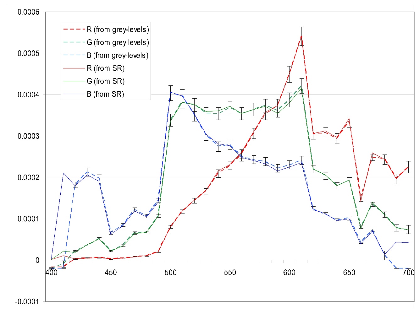
Figure 2 below shows a comparison of the energy flux calculations across the spectrum (31 narrowband filters) using the two methods, radiometrically-based and model-based. Both estimates reach good agreement considering the error bars (based on the StdDev of the grey-level counts r,g,b).
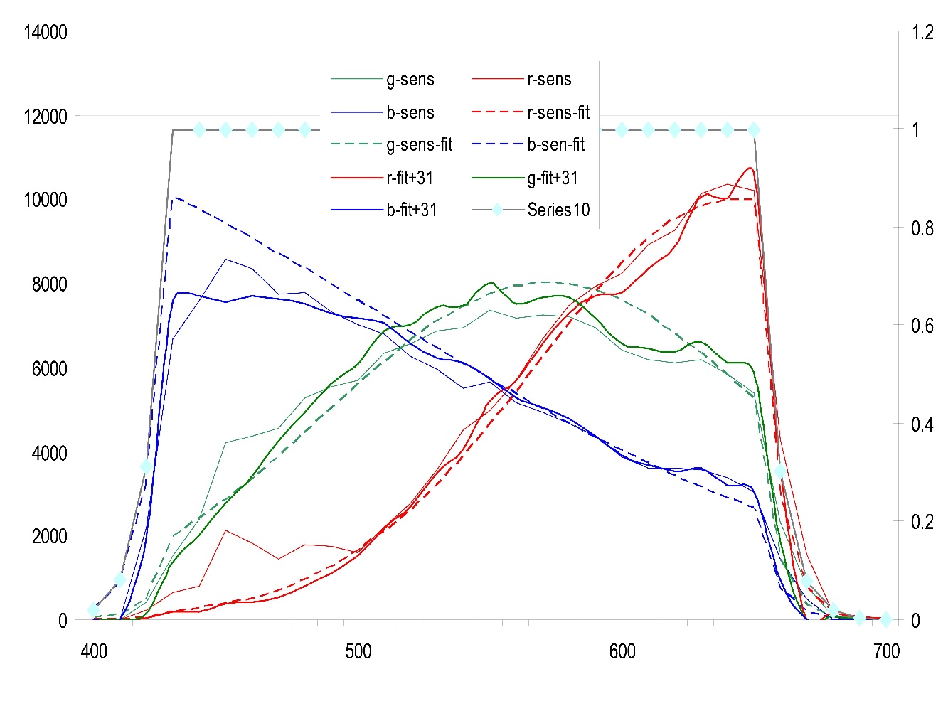
To obtain the agreement shown in Figure 2, the shape of S(l) was modified from the original Gaussians (for each colour channel) allowing each point to fluctuate a fixed percentage around the starting values. Figure 3 below shows the final shape of the sensor sensitivity functions, SR(l), SG(l) and SB(l), obtained after being adjusted so that equations 9 are minimised. The parameters obtained from the fittings were:
|
a |
b |
c |
d |
red |
1.3176.10-7 |
1.1949 |
-2.503·10-4 |
-601.7059 |
green |
1.7044.10-7 |
1.2603 |
-4.2848·10-4 |
-911.0773 |
blue |
1.9233.10-7 |
1.2671 |
-3.2769.10-4 |
-680.8141 |
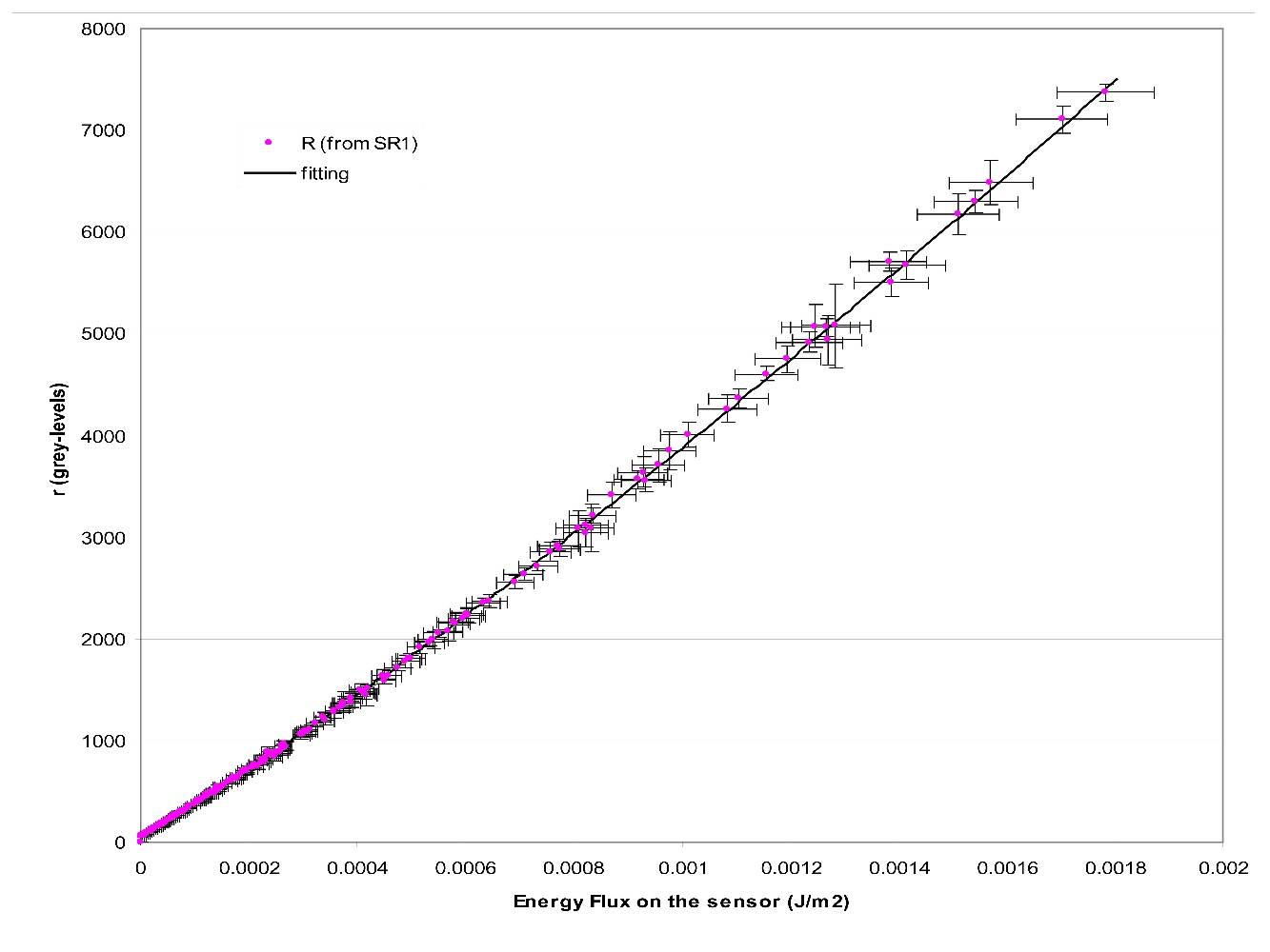
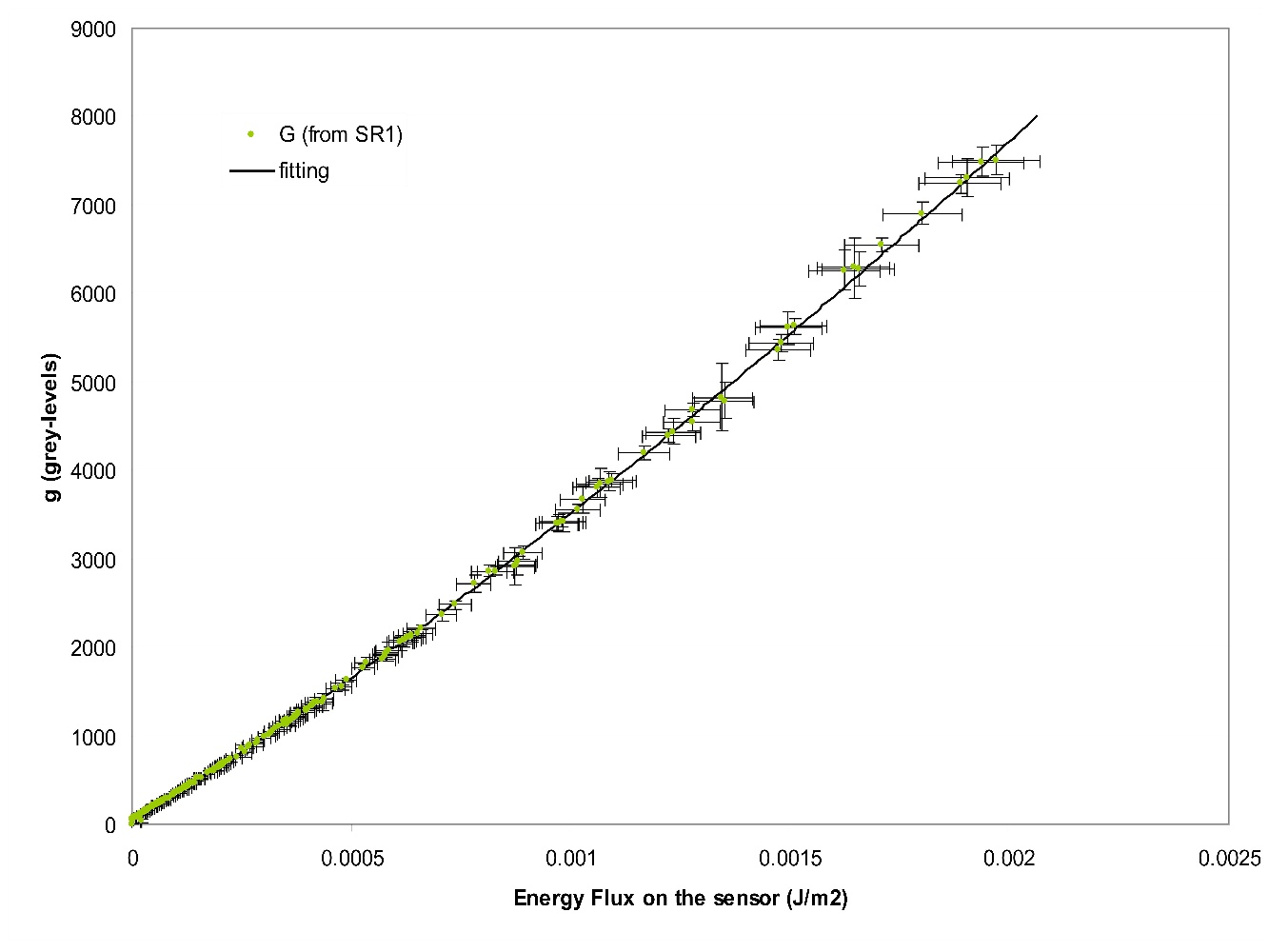
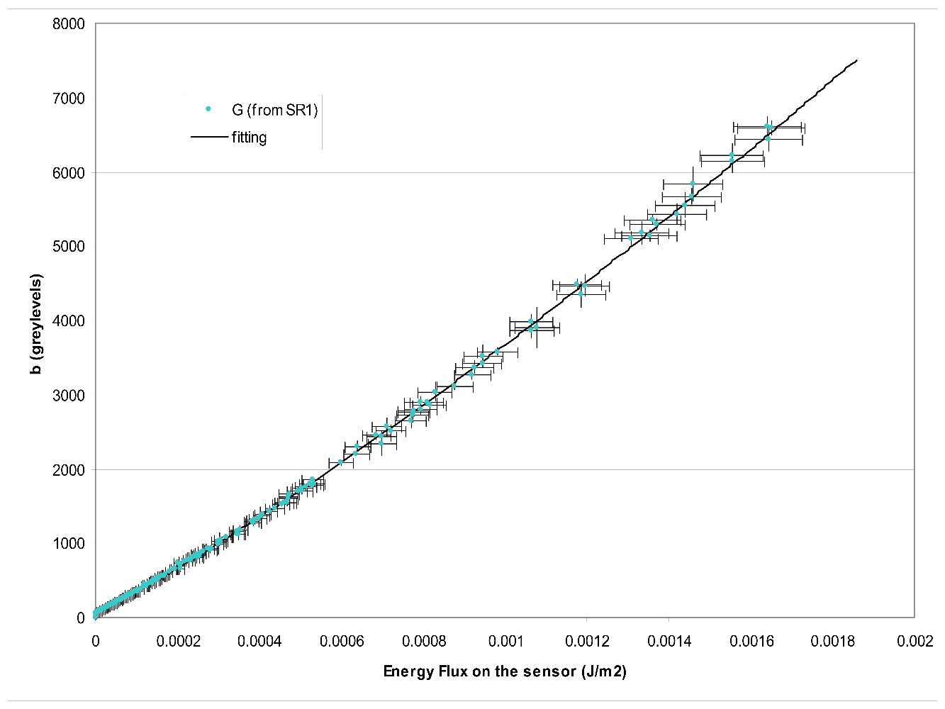
and now it is possible to confirm the relationship between the grey-level output (r,g,b) and the energy flux on the sensors. The results can be seen below (Figure 4, Figure 5 and Figure 6) for the red, green and blue sensors respectively.
