Space Conversions

Camera to CIE XYZ conversions: an ill-posed problem

For our pictures to be truly useful for scientific research they need to be specified in a standardised colour system. One of the most widely used colour systems is the one specified by the CIE (1931) standard observer. The main reason for this is because there are several widely available transforms / algorithms that can translate the CIE 1931 tristimulus values into any other colour space. That is the main reason we have decided to specify out pictures in CIE (1931) XYZ format.

However, there are strong constraints to the maximum precision to which we can specify the colours captured by the camera's sensors, simply because there is no guarantee that a single colour transformation will allow us to convert all possible colours from the device-dependent camera space to the device-independent CIE (1931) space. These constraints are illustrated by Figure 1 (below), where a single transformation between the ABC and the PQR systems is clearly impossible. In fact we found that for our particular case (see Figure 2), there isn't any (ill-posed problem). We could find a transformation that works approximately well for the majority of colours, or we could try to optimise the transformation for some interesting colours (such as the colours most commonly found in nature or the colours most commonly found in urban environments, etc.). There are statistical-based approaches where a set of colours is measured and photographed and a transformation is found to best suit those colours. The problem with this approach (that works best for the "learnt" colours) is that to optimise for a different dataset we need to run the measurements again. However, we have an interesting advantage: we know the internal workings of our camera (or at least we have sort of modeled them) and we can devise a simple way of optimising our colour conversions to the set of colours that we are interested in photographing. For example, we know that our dataset will contain pictures of natural objects and colours (such as sky, earth, bark, chlorophyll, flowers, etc) and there are publicly available databases of radiometric samples of those colours, which can be used to predict the camera's RGB output (using the camera model) and whose XYZ values are known or can be calculated. Then we can build the optimal theoretical transformation from the camera system to the XYZ system to process those images. This is where the advantages of having a properly calibrated camera come to play an important role.

The choice of transformation functions

There are many ways to transform the output from a set of sensor sensitivities like ours to another, like the CIE XYZ system. The most common transform consists on finding a 3x3 matrix that would do the trick:

RGBtoXYZ 3x3 matrix

Where X,Y,Z are the tristimulus values of the CIE (1931) colour system and R,G,B are the values (quantal catch) obtained from our camera model. The 3x3 conversion matrix M is relatively easy to obtain, doing:

M= CIEXYZ' * (Sensors);

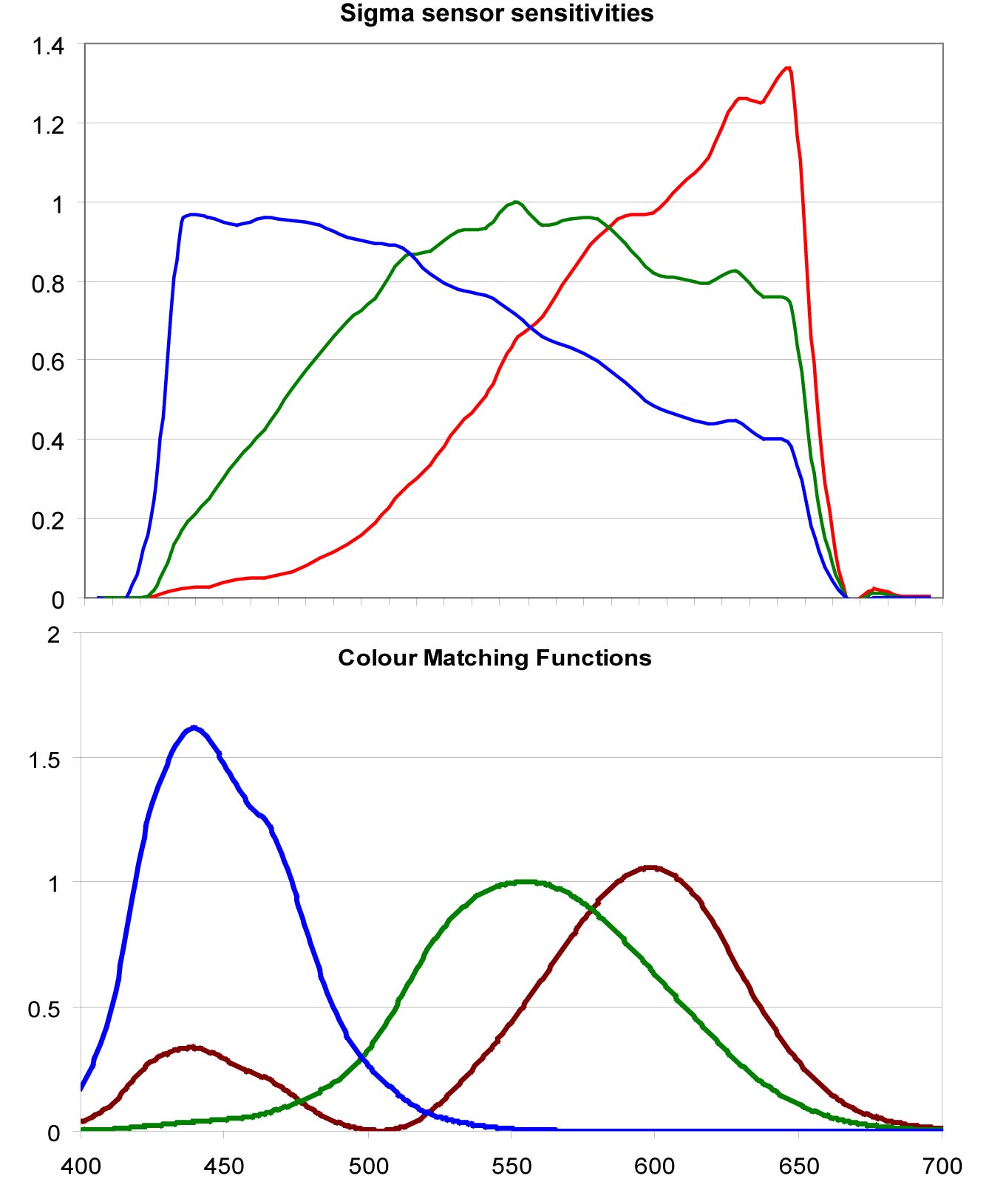
where CIEXYZ is the (31x3) matrix of CIE1931 Colour Matching Functions and Sensors are the (31x3) sensor sensitivity functions of the camera. Figure 3 (below) shows the results of comparing the XYZ values obtained by using the simple matrix transformation above to those measured by the spectroradiometer for all 24 Macbeth patches at photographed at 10 different integration times. The results (especially for the blue sensor) are not very encouraging. As mentioned before a simple 3x3 matrix transformation cannot capture the complexity of the problem.

A second approach consists on adjusting the values of M to fit the calculated data to the measured data. Figure 4 shows the results from this approach

A third approach consisted on replacing the 3x3 matrix by a polynomial function of the form:

poly definition

Where K is also defined in terms of aperture, focal length and integration time and the coefficients M are determined by fitting the data to some known dataset. The advantages of defining parameters M in terms of the type of data we want to photograph becomes evident in the example below. Suppose we want to adjust our camera output so that it matches all colours defined in the Munsell chart (their spectral reflectances are easily available). We could calculate the RGB values that such colours would produce when illuminated by a standard light and photographed by our camera (in theory), calculate their XYZ values using the CIE 1931 colour matching functions and then find the best set of parameters M for those values. This will provide a universal solution, adjusted to all colours and containing large errors in some parts of the colour space. Now suppose we are interested in just a sub-sample of all the colours of the world such as the most common colours present in nature. Then we could repeat the procedure using a database of spectral reflectances of natural objects and natural illuminations (which are also available). Then our camera RGB-to-XYZ transformation would be optimised for those combinations of colours and illuminations. Figure 5 (below) shows a comparison of the XYZ values obtained from the Macbeth card by our camera model after parameters M were optimised for the whole of the Munsell book. Similarly, Figure 6 was obtained with the camera optimised for a database of Northern-European natural reflectances (Parkkinen et al ``Spectral representation of colour images,'' IEEE 9th International Conference on Pattern Recognition, Rome, Italy, 14-17 November, 1988, Vol. 2, pp. 933-935. ).

The Matlab functions used to convert from camera space to CIE XYZ space are here.

1. Extreme example of our ill-posed problem The figure below was constructed for illustrative purposes and shows an extreme case where the conversion between two colour systems is highly inaccurate. Suppose we have a camera with spectral sensitivities ABC and we want to convert its output to a colour system specified by the PQR functions. Since the two systems hardly overlap, the transformation will be undetermined.

ABC to PQR

2. The actual problem: from camera system to XYZThe figure below shows the actual problem presented when we try to transform colours as determined by the camera's sensors to those described by the CIE (1931) system: our problem is ill-posed, there isn't a single transformation that is valid for all possible colours.

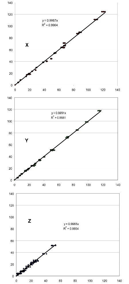3. Simple matrix transformation Comparison of the XYZ values obtained by using the simple matrix transformation (displayed on the abscissas) against those measured by the spectroradiometer (displayed on the ordinates) for all 24 Macbeth patches at photographed at 10 different integration times. Plots correspond to each of the X, Y and Z tristimulus values.

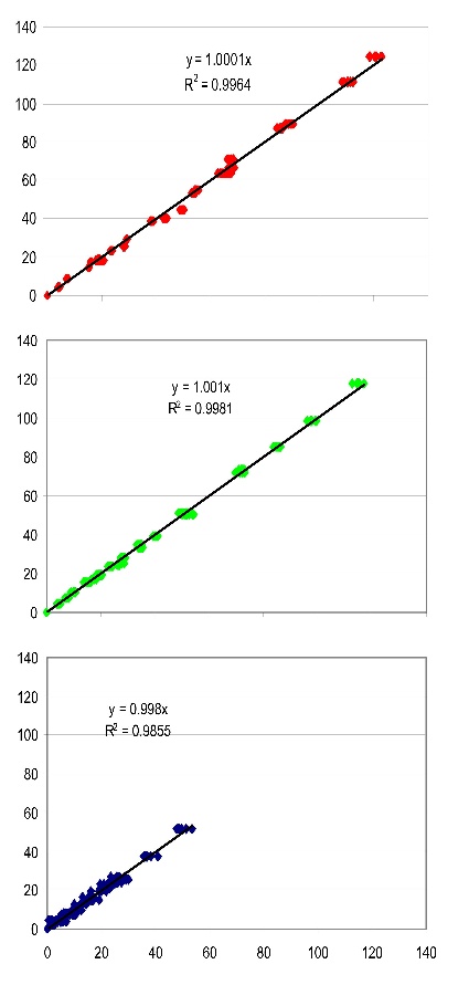4. Adjusted matrix transformation Simple Matrix Comparison of the XYZ values obtained by using the adjusted polynomial transformation (displayed on the abscissas) against those measured by the spectroradiometer (displayed on the ordinates) for all 24 Macbeth patches at photographed at 10 different integration times. Plots correspond to each of the X, Y and Z tristimulus values. The polynomial parameters were adjusted to optimally fit the Macbeth chart data. Plots correspond to each of the X, Y and Z tristimulus values.

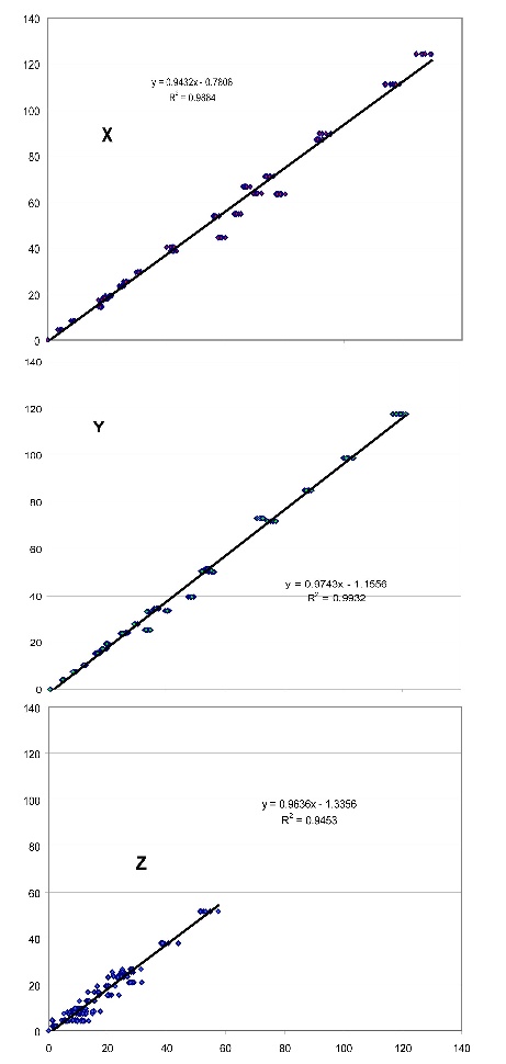5. Adjusted to the Munsell book Simple Matrix Comparison of the XYZ values obtained by using the polynomial transformation (displayed on the abscissas) against those measured by the spectroradiometer (displayed on the ordinates) for all 24 Macbeth patches at photographed at 10 different integration times. The polynomial parameters were adjusted to optimally match the Munsell book data. Plots correspond to each of the X, Y and Z tristimulus values.

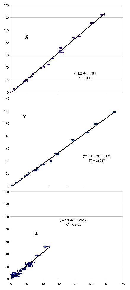6. Adjusted to Northern Europe natural reflectances Simple Matrix Comparison of the XYZ values obtained by using the polynomial transformation (displayed on the abscissas) against those measured by the spectroradiometer (displayed on the ordinates) for all 24 Macbeth patches at photographed at 10 different integration times. The polynomial parameters were adjusted to optimally match a database of natural objects' reflectances data. Plots correspond to each of the X, Y and Z tristimulus values.

Centre de Visió per Computador - Universitat Autònoma de Barcelona

Colour space conversion

Related Links

Other image databases

Camera to CIE XYZ conversions: an ill-posed problem

The choice of transformation functions