A simple trichromatic camera model
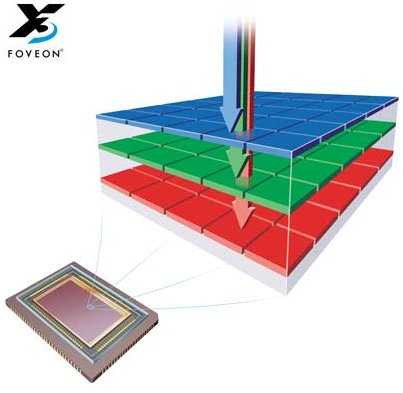
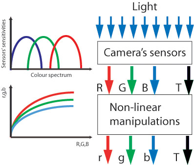
We modeled our trichromatic imaging device as a set of three sensors (first, linear module), each responding to a given portion of the electromagnetic spectrum, with spectral sensitivities that largely overlap. This first module produces an output labeled R, G and B (see figure). The second transformation correspond to a non-linear module which converts the sensor’s output (RGB) into r, g and b values (grey-levels) to create the three final components of a colour image. At this stage we can think of R, G, and B as internal representations of the total energy captured by each sensor, and r, g, and b as the grey-levels that define each individual pixel in the final image.
We selected the camera settings so that the integration time (referred here as T, a.k.a. the inverse of the shutter speed) is calculated automatically by the camera to keep the amount of energy falling onto the sensors within their dynamic range (most pixels are neither "too dark" or "saturated"). This integration time T is recorded in the picture header. The figure below shows the schematics of such model.
 The criterion by which the second (non-linear) module modifies the output of the first module depends on the manufacturer (who may consider primarly the cosmetic appearance of the final image and the characteristics of the final presentation device i.e. printer, monitor, etc). There is also some kind of illumination compensation mechanism, usually called "white balance" so that the final picture reflects approximately the observer’s impression (which is defined by our brain's tendency to get rid of the colour of the illumination). This mechanism may be automatic or manual (i.e. the user must enter the type of illumination under which the picture was taken) and generally adds a differential “gain factor” to each of the RGB channels in the second module to approximately match the characteristics of the presentation device and provide a cosmetically acceptable image. The algorithms used by the camera manufacturer to reach the final output are in general unknown. Assuming that the overall behaviour of the sensors with intensity is the same, we could just look at one of the three sensors (e.g. the middle-wavelength or green) and use it as template. The relationship between the green sensor's output and the light shinning on it can be expressed as:
| :Equation 1 |
|---|
where g is the grey-level value of a given pixel plane (e.g. the green pixel plane), E is the energy captured by the sensor (which in turn depends of its spectral sensitivity, the inegration time and some geometrical factors of the camera optics like as aperture and focal length). In this analysis we will ignore smallish artifacts (such as spatial inhomogeneity of the image caused by lens aberrations, the MTF of the lens, etc.), assuming that R, G and B are strictly dependent of the incoming spectral radiance. These will be dealt with by the subsequent tunning of the model's parameters to experimental data.
If the green sensor sensitivity S(λ) was the same as the CIE (1931) ![]() colour matching function, we could write E in terms of Luminance (L).
colour matching function, we could write E in terms of Luminance (L).
if S(λ) = ![]() (λ), then:
(λ), then:
 |
:Equation 2 | |
|---|---|---|
where E is the energy flux (Joules m-2) incident on the sensor, f is the camera's aperture ratio (the ratio between its focal length l and aperture a, represented by the camera’s F-stop number), T is the integration time as obtained from the pictures' headers, K is the maximum luminous efficacy of radiant power (683 lm/W) and L is luminance.
A simplification like the one proposed above would make our life much simpler because then:
| :Equation 3 |
|---|
g would be just a function of Luminance. But life is usually more complicated than that.
First estimation of the camera’s non-linearities
The main problem with our estimation of the relationship f is the dependence of E (total energy captured by the sensor) on the sensor's sensitivity S(λ), which is an unknown function of wavelength . Suppose we take a series of pictures of a given target (of known radiance) at different illumination levels and plot g as a function of radiance. We still do not know what part of this radiance spectrum is captured by the sensor!. If we had a equal-energy illuminant (the same spectral radiance at any given wavelength) we may be able to estimate how much each R, G, or B sensor is collecting relative to the others, but we still don't know their spectral sensitivities.
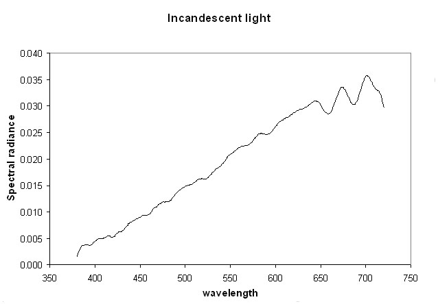
However, it is possible to estimate the shape of the relationship between sensor output and light intensity by assuming that the green sensor's Sg(λ) has a shape similar to the CIE (1931) ![]() colour matching function and spans over a similar part of the visual spectrum. This assumption seems to be reasonable as a starting point since it would make sense for camera manufacturers to approximate the output of middle-wavelength sensor to a linear function of luminance. However, our experimental setup (see below) uses an incandescent light source, which radiates more energy in the long-wavelength (reddish) part of the visible spectrum than in the short-wavelength (bluish) part and without knowing the corresponding sensor’s sensitivities for Sr(λ) and Sb(λ) it is not possible to work out their exact relationships to light intensity.
colour matching function and spans over a similar part of the visual spectrum. This assumption seems to be reasonable as a starting point since it would make sense for camera manufacturers to approximate the output of middle-wavelength sensor to a linear function of luminance. However, our experimental setup (see below) uses an incandescent light source, which radiates more energy in the long-wavelength (reddish) part of the visible spectrum than in the short-wavelength (bluish) part and without knowing the corresponding sensor’s sensitivities for Sr(λ) and Sb(λ) it is not possible to work out their exact relationships to light intensity.
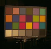
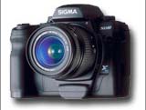
 To estimate the relationship between light intensity and camera output, we illuminated a Macbeth ColorChecker colour rendition card with incandescent light (see figure on the left and detailed methods below) and obtained both, the radiometric measures of the central part of the bottom row of squares and the average pixel value (and corresponding StdDev.). Ten different pictures were taken at ten different integration times (ranging from 0.32 to 2.59 sec). Saturated or dark (noisy) values were discarded. Following the initial supposition that the camera green sensor was collecting energy in about the same spectral region as the CIE (1931)
 ![]() colour matching function, we estimate the energy flux I (in Joules m-2) captured by the sensor using equation 2.
colour matching function, we estimate the energy flux I (in Joules m-2) captured by the sensor using equation 2.
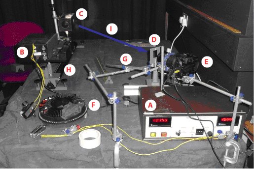
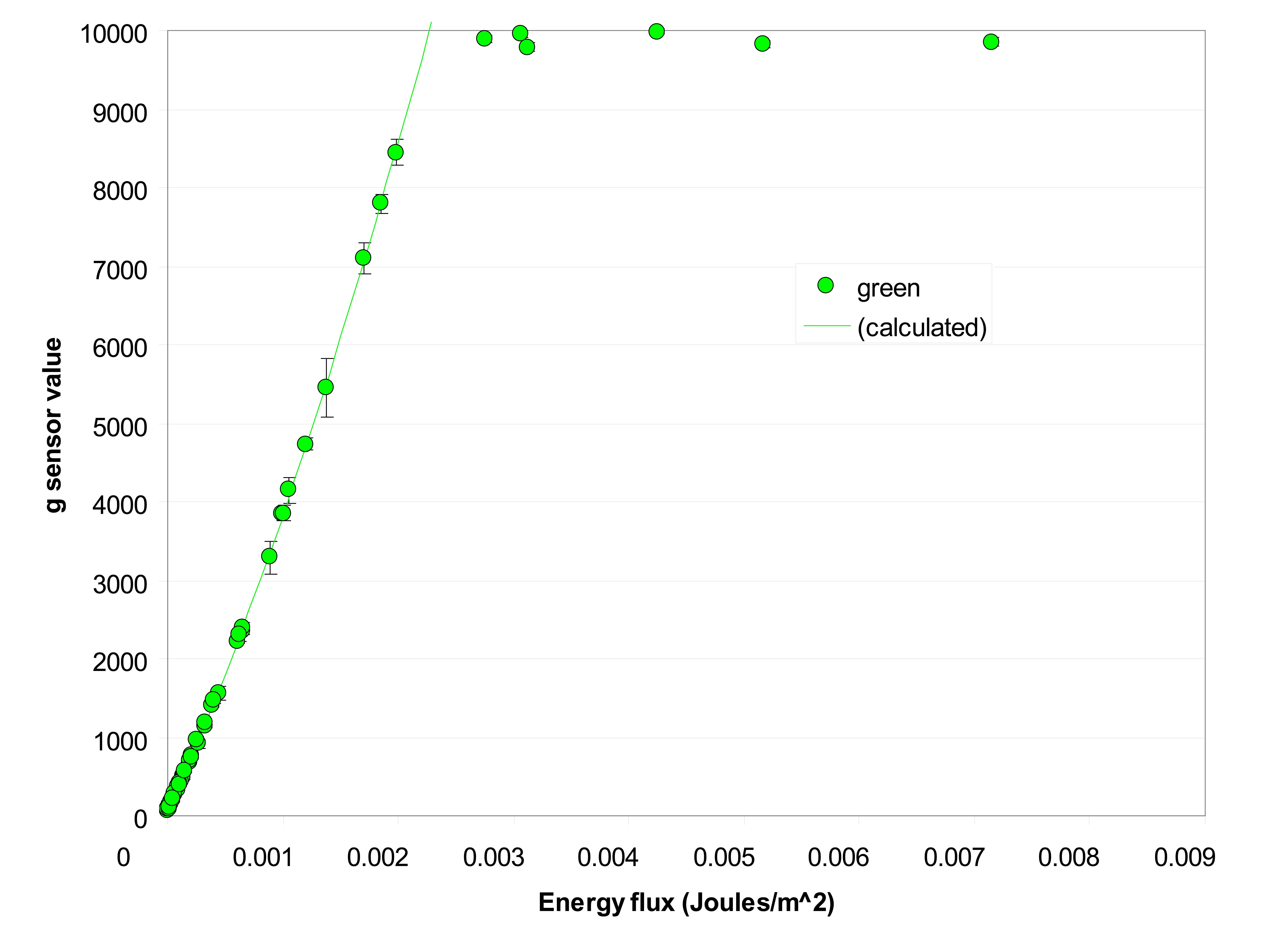
In our particular case, h (the camera's aperture) was 5 mm, l (the focal length) was 35 mm, and K is the maximum luminous efficacy of radiant power (683 lm/W). L is the luminance measured by the spectroradiometer and T (integration time) was obtained from the pictures' headers. The camera settings were chosen for best convenience, since a small aperture provides the bigger depth of field that is needed in most naturalistic photography. The figure above shows the relationship between the measured energy flux (E) and the corresponding pixel grey-levels. Notice that despite the manufacturer's claim that the camera provides sensitivities of 16-bit per sensor, we could not obtain values of g larger than 10,000 (less than 14-bit) because of saturation. Still, this is significantly bigger than the usual 8-bit per sensor of commercial digital cameras.
The following function was fitted to the measured data:
| :Equation 4 |
|---|
where G is the picture grey-level for the green sensor,E is the Energy flux and a, b, c and d are free parameters. As a first step, we assumed a similar relationship to be valid for the other two sensors (red and blue). This function (which is similar to the "gamma function" of CRT monitors) was chosen not only because it fits the data appropriately but also because it is reversible (see next steps).
Equation 4 gives us an estimation (remember that it was obtained by supposing that the spectral sensitivity of our sensor is the same as the CIE ![]() colour matching function!) of the dependency between grey-level and energy flux for the green sensor of the Foveon SD10. However, it will allow us to carry on with the next step of our camera calibration.
colour matching function!) of the dependency between grey-level and energy flux for the green sensor of the Foveon SD10. However, it will allow us to carry on with the next step of our camera calibration.