Chromaticity under incandescent lighting
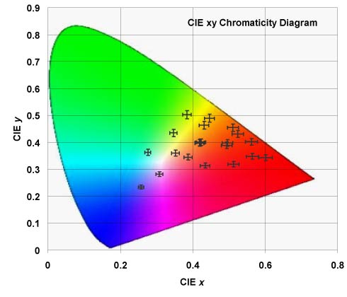
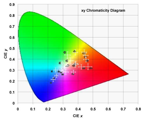
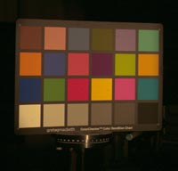 Figure 1(below) shows a CIE diagram with the points corresponding to each square of the Macbeth Card as measured by the spectroradiometer (circles) and the equivalent measure from our camera (crosses). The values are shifted towards red because of the colour of the incandescent illuminant.
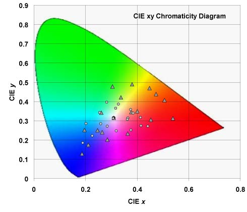
If we scale the same data so that square 21 (neutral 6.5) has exactly the same values as stated by the card's manufacturers, all points move nearer the centre of the plot (low saturation). When we look at these results we notice that the xy chromaticity values obtained by scaling the spectroradiometric measures do not match those advertised by the card's manufacturer. This may be due to fainting/aging of the card and the angle of incidence of the light. To have an idea of the effects of this "fainting" on the Macbeth card, Figure 2 shows a plot of the chromaticity values of the Macbeth card as expected from the manufacturer's statement (filled circles) and as measured by our spectroradiometer (empty circles). This card is an older card used for the calibration and shown above under incandescent illumination. The second card (shown under natural illumination) used for the tests is much newer and we expect the "fainting" effect to be less extreme. To properly test our camera model, the chromaticity values of the card under natural illumination have to be measured (as opposed to believing the manufacturer's claims).
Chromaticity under Natural Illumination
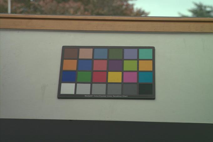 To establish how accurate are the measurements provided by the camera model is not straightforward. The main problem is that our model has been optimised to represent the colours used during the calibration process (macbeth card colours under incandescent illumination) and most of the pictures we are interested do not have a similar distribution of colours and furthermore, they are under natural illumination. The answer is to photograph the Macbeth card under daylight illumination and then compare the results to some sort of measurement... However, since natural illumination is not constant, and the spectroradiometer can only measure one colour at the time, we need to photograph and measure each colour at the same time!
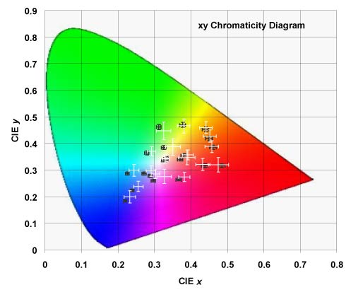
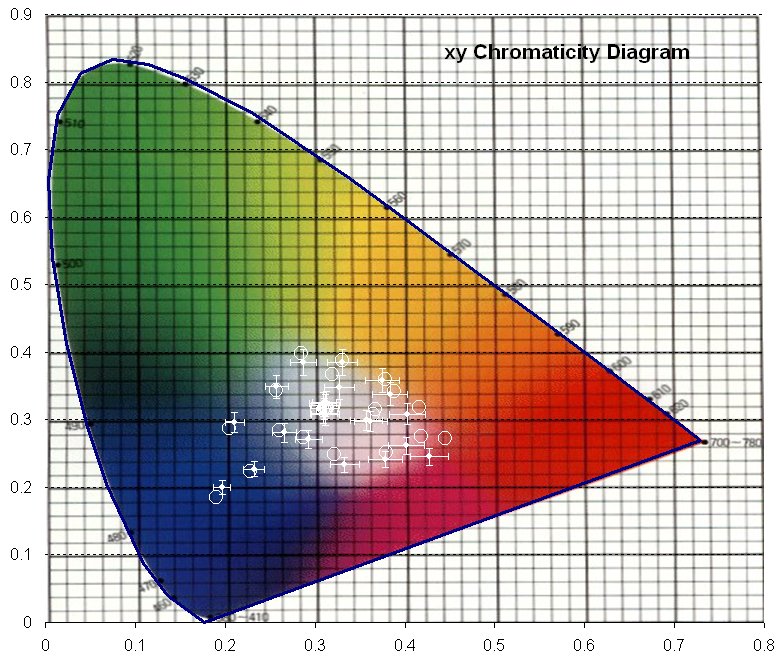
To overcome this problem, we arranged the system so that both the camera and the spectroradiometer receive light reflected from the card at similar angles, record their measures from the same distance and at the same time. To achieve an approximate timing of the camera and the spectroradiometer we shot both instruments at the same time, thus obtaining 24 XYZ measures and 24 pictures taken with our camera. The aperture was the same for all images and we let the camera choose the best integration time to suit changes in lighting. The illumination however was very stable (it was a typical autumn cloudy day in the English West Country). Figure 3 shows a plot of the the CIE chromaticity values (white crosses) and the corresponding spectroradiometric measurements (grey crosses). The model used was the generalist "adjusted to Munsell book" variant (see here for an explanation). The size of the white crosses represent the StdDev of the estimation obtained from the camera, since each square sample consisted on a circular selection of the central section of each square where pixels had different values, thus an statistical mean was obtained. The corresponding grey crosses represent the uncertainty obtained from the spectroradiometric measures (also obtained from the approximate centre of each coloured square) which was determined to be about 3% the last time this instrument was calibrated by the UK National Physics Laboratory. As Figure 3 shows, the output of the camera model corresponds quite closely to that of the spectroradiometer (except perhaps in the "bluish" side of the plot) within their corresponding error measures (the average Euclidean distance between the two measures is 0.014). The same is the case for the "adjusted to Northern European colours " variant of the model (average euclidean distance equal to 0.017) whose results are shown in Figure 5. The Table below provides a numerical description of the values presented in Figures 3 and 5, i.e. the spectroradiometer chromaticity results, and the model's results on its two variations (Munsell-book and NE).
patch name |
SR measurements |
Camera model |
||||||
Munsell book optimisation |
NE dataset optimisation |
|||||||
x |
y |
x |
y |
x |
y |
|||
| dark skin | 0.371 |
0.341 |
0.389 |
0.348 |
0.382 |
0.351 |
||
| light skin | 0.381 |
0.355 |
0.392 |
0.357 |
0.385 |
0.360 |
||
| blue sky | 0.272 |
0.287 |
0.291 |
0.297 |
0.289 |
0.300 |
||
| foliage | 0.326 |
0.385 |
0.351 |
0.387 |
0.349 |
0.385 |
||
| blue flower | 0.289 |
0.279 |
0.302 |
0.285 |
0.298 |
0.290 |
||
| bluish green | 0.279 |
0.364 |
0.292 |
0.370 |
0.295 |
0.364 |
||
| orange | 0.461 |
0.386 |
0.458 |
0.389 |
0.453 |
0.396 |
||
| purplish blue | 0.239 |
0.224 |
0.256 |
0.239 |
0.256 |
0.248 |
||
| moderate red | 0.438 |
0.317 |
0.433 |
0.321 |
0.422 |
0.329 |
||
| purple | 0.297 |
0.260 |
0.327 |
0.276 |
0.319 |
0.283 |
||
| yellow green | 0.378 |
0.470 |
0.381 |
0.466 |
0.383 |
0.461 |
||
| orange yellow | 0.450 |
0.419 |
0.452 |
0.428 |
0.450 |
0.433 |
||
| blue | 0.220 |
0.184 |
0.233 |
0.199 |
0.235 |
0.214 |
||
| green | 0.312 |
0.462 |
0.326 |
0.448 |
0.330 |
0.437 |
||
| red | 0.485 |
0.317 |
0.476 |
0.320 |
0.466 |
0.330 |
||
| yellow | 0.440 |
0.454 |
0.441 |
0.460 |
0.442 |
0.463 |
||
| magenta | 0.367 |
0.265 |
0.383 |
0.274 |
0.370 |
0.283 |
||
| cyan | 0.226 |
0.287 |
0.244 |
0.300 |
0.251 |
0.301 |
||
| white | 0.333 |
0.343 |
0.332 |
0.345 |
0.328 |
0.345 |
||
| neutral 8 | 0.326 |
0.338 |
0.329 |
0.342 |
0.326 |
0.342 |
||
| neutral 6.5 | 0.322 |
0.334 |
0.326 |
0.343 |
0.323 |
0.343 |
||
| neutral 5 | 0.317 |
0.331 |
0.322 |
0.338 |
0.319 |
0.338 |
||
| neutral 3.5 | 0.312 |
0.321 |
0.321 |
0.338 |
0.318 |
0.338 |
||
| black | 0.312 |
0.325 |
0.312 |
0.343 |
0.311 |
0.342 |
||
it is important to realise that the error committed by the camera and the spectroradiometer (Figures 3 and 5) are much smaller than the error caused by taking the macbeth card manufacturer's values for granted! (Figure 2). These values are highly dependent on the manufacture date of the card, angle of incidence of light, etc.
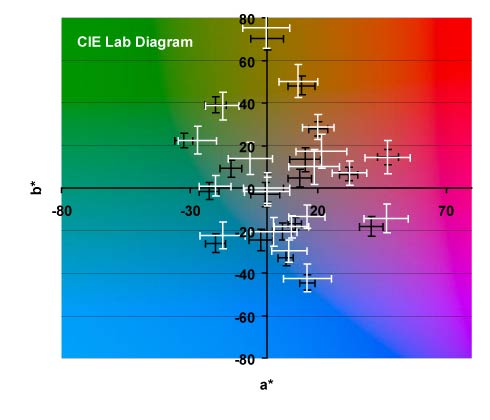
The last two figures show the same values in the (more perceptually uniform) Lab space. The error bars represent measurement errors propagated though the XYZ-to-Lab conversion equations.
The matlab functions used to convert from the camera space to the CIEXYZ space are here.
